LDA

My Undergraduate Thesis is about LDA, Exploring the hidden factors online food shopping from Amazon reviews by LDA

Now, let me sum up LDA again.

LDA (latent Dirichlet allocation) is a topic model, which can give the topic of each document in the document set in the form of probability distribution. At the same time, it is an unsupervised learning algorithm, which does not need manual annotation of the training set, but only the document set and the number of specified topics K. Another advantage of LDA is that it can find some words to describe each topic. LDA was first proposed by BLEI, David M., Wu Enda and Jordan, Michael I in 2003. At present, LDA has applications in text mining, including text topic recognition, text classification and text similarity calculation.

We describe latent Dirichlet allocation (LDA), a generative probabilistic model for collections of discrete data such as text corpora. LDA is a three-level hierarchical Bayesian model, in which each item of a collection is modeled as a finite mixture over an underlying set of topics. Each topic is, in turn, modeled as an infinite mixture over an underlying set of topic probabilities. In the context of text modeling, the topic probabilities provide an explicit representation of a document. We present efficient approximate inference techniques based on variational methods and an EM algorithm for empirical Bayes parameter estimation. We report results in document modeling, text classification, and collaborative filtering, comparing to a mixture of unigrams model and the probabilistic LSI model.

from Latent Dirichlet Allocation DM Blei, AY Ng, MI Jordan - Journal of Machine Learning Research 3 (2003)

\[p(w_{i},z_{i},\theta _{i},\Phi |\alpha ,\beta )=\prod _{j=1}^{N}p(\theta _{i}|\alpha )p(z_{i,j}|\theta _{i})p(\Phi |\beta )p(w_{i,j}|\phi _{z_{i,j}})\]

You need to learn these knowledage firstly before study:

Bayes’ theorem basic

\[p(\theta|x)={p(x|\theta)p(\theta)\over p(x)}\]

Prior probability

\[p(\theta)\]

Posterior probability

\[p(\theta|x)\]

Likelihood

\[p(x|\theta)\]

Conjugate prior

pdf

pdf(k, mu, loc=0, scale)

Probability density function

\[f(x)={\frac {\partial ^{n}F}{\partial x_{1}\cdots \partial x_{n}}}{\bigg |}_{x}\]

cdf

cdf(k, mu, loc=0, scale)

Cumulative distribution function.

\[F(x) = \int_{-\infty }^{x}f(x)\,dt\]

Cumulative distribution function’s derivative can be used as probability density function

pmf

pmf(k, mu, loc=0)

Probability mass function

Binomial distribution

\[f(k,n,p)=P(X=k)={n \choose k}p^{k}(1-p)^{n-k}\]

In probability theory and statistics, binomial distribution is a discrete probability distribution of n independent yes / no test success times, in which the success probability of each test is p. Such a single success / failure test is also known as the Bernoulli test. In fact, when n = 1, binomial distribution is Bernoulli distribution. Binomial distribution is the basis of two experiments with significant difference.

scipy.stats.binom

from scipy.stats import binom
import matplotlib.pyplot as plt
import numpy as numpy

fig, ax = plt.subplots(1, 1)
n, p = 5, 0.4
#moments(矩)
mean, var, skewm, kurt = binom.stats(n, p, moments = 'mvsk')
#Display the probability mass function(pmf)
x = np.arange(binom.ppf(0.01, n, p), binom.ppf(0.99, n, p))
ax.plot(x, binom.pmf(x, n, p), 'bo', ms = 8, label = 'binom pmf')
ax.vlines(x, 0, binom.pmf(x, n, p), colors = 'b', lw = 5, alpha = 0.5)
rv = binom(n, p)
ax.vlines(x, 0, rv.pmf(x), colors = 'k', linestyles = '-', lw = 1, label = 'frozen pmf')
ax.legend(loc = 'best', frameon = False)
plt.show()

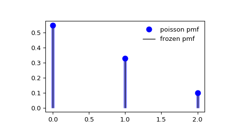
Poisson distribution

\[P(X=k)=\frac{\lambda^k}{k!}e^{-\lambda}\]

The number of such events that occur during a fixed time interval is, under the right circumstances, a random number with a Poisson distribution.

such as the number of laser photons hitting a detector in a particular time interval

The Poisson distribution is also the limit of a binomial distribution, for which the probability of success for each trial equals λ divided by the number of trials, as the number of trials approaches infinity

scipy.stats.poisson

from scipy.stats import poisson
import matplotlib.pyplot as plt
import numpy as numpy

fig, ax = plt.subplots(1, 1)

mu = 0.6
mean, var, skew, kurt = poisson.stats(mu, moments='mvsk')
x = np.arange(poisson.ppf(0.01, mu),
              poisson.ppf(0.99, mu))
ax.plot(x, poisson.pmf(x, mu), 'bo', ms=8, label='poisson pmf')
ax.vlines(x, 0, poisson.pmf(x, mu), colors='b', lw=5, alpha=0.5)
rv = poisson(mu)
ax.vlines(x, 0, rv.pmf(x), colors='k', linestyles='-', lw=1,
        label='frozen pmf')
ax.legend(loc='best', frameon=False)
plt.show()

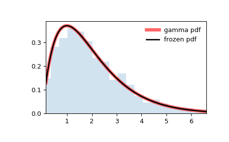
Gamma distribution

\[\Gamma(x) = \int_0^\infty t^{x-1}e^{-t}dt\] \[\Gamma(n) = (n-1)!\]

In probability theory and statistics, the gamma distribution is a two-parameter family of continuous probability distributions.

From the point of view of significance: the problem solved by the exponential distribution is “how long does it take to wait for a random event to happen”, and the problem solved by the gamma distribution is “how long does it take to wait for N random events to happen”.

scipy.stats.gamma

from scipy.stats import gamma
import matplotlib.pyplot as plt
import numpy as numpy

fig, ax = plt.subplots(1, 1)
a = 1.99
mean, var, skew, kurt = gamma.stats(a, moments='mvsk')
#Display the probability density function (pdf):

x = np.linspace(gamma.ppf(0.01, a),
                gamma.ppf(0.99, a), 100)
ax.plot(x, gamma.pdf(x, a),
       'r-', lw=5, alpha=0.6, label='gamma pdf')

rv = gamma(a)
ax.plot(x, rv.pdf(x), 'k-', lw=2, label='frozen pdf')
vals = gamma.ppf([0.001, 0.5, 0.999], a)
np.allclose([0.001, 0.5, 0.999], gamma.cdf(vals, a))
#Generate random numbers
r = gamma.rvs(a, size=1000)
ax.hist(r, density=True, histtype='stepfilled', alpha=0.2)
ax.legend(loc='best', frameon=False)
plt.show()

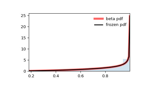
Beta distribution

\[\begin{align} f(x; \alpha, \beta) = \frac{1}{B(\alpha, \beta)} x^{\alpha - 1} {(1-x)}^{\beta-1} \end{align}\] \[\begin{align} \frac{1}{B(\alpha, \beta)} = \frac{\Gamma(\alpha + \beta)}{\Gamma(\alpha)\Gamma(\beta)} \end{align}\]

Conjugate prior of binomial distributions

You can understand it as observing the probability distribution of a group of experiments from different angles. The beta distribution is to study the distribution of theta given a set of data x, while the binomial distribution is to study the distribution of X given theta

scipy.stats.beta

from scipy.stats import beta
import matplotlib.pyplot as plt
import numpy as numpy

fig, ax = plt.subplots(1, 1)
a, b = 2.31, 0.627
mean, var, skew, kurt = beta.stats(a, b, moments='mvsk')
x = np.linspace(beta.ppf(0.01, a, b),
                beta.ppf(0.99, a, b), 100)
#pdf: Probability density function.
ax.plot(x, beta.pdf(x, a, b),'r-', lw=5, alpha=0.6, label='beta pdf')
rv = beta(a, b)
ax.plot(x, rv.pdf(x), 'k-', lw=2, label='frozen pdf')
#ppf: Percent point function (inverse of cdf — percentiles)
vals = beta.ppf([0.001, 0.5, 0.999], a, b)
np.allclose([0.001, 0.5, 0.999], beta.cdf(vals, a, b))
#Generate random numbers
r = beta.rvs(a, b, size=1000)
ax.hist(r, density=True, histtype='stepfilled', alpha=0.2)
ax.legend(loc='best', frameon=False)
plt.show()

Expectation

\[\mu =\operatorname {E}(X)={\frac {\alpha }{\alpha +\beta }}\]

Variance

\[\operatorname {Var}(X)=\operatorname {E}(X-\mu )^{2}={\frac {\alpha \beta }{(\alpha +\beta )^{2}(\alpha +\beta +1)}}\]

Skewness

\[\frac{2\,(\beta-\alpha)\sqrt{\alpha+\beta+1}}{(\alpha+\beta+2)\sqrt{\alpha\beta}}\]

scipy.stats.skew

from scipy.stats import skew
skew([2, 8, 0, 4, 1, 9, 9, 0]) #return 0.2650554122698573

Kurtosis

\[{\frac {\operatorname {E}(X-\mu )^{4}}{[\operatorname {E}(X-\mu )^{2}]^2}}-3={\frac {6[\alpha ^{3}-\alpha ^{2}(2\beta -1)+\beta ^{2}(\beta +1)-2\alpha \beta (\beta +2)]}{\alpha \beta (\alpha +\beta +2)(\alpha +\beta +3)}}\]

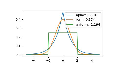
scipy.stats.kurtosis

import scipy.stats as stats
from scipy.stats import kurtosis
import matplotlib.pyplot as plt
import numpy as np

x = np.linspace(-5, 5, 100)
ax = plt.subplot()

distnames = ['laplace', 'norm', 'uniform']
for distname in distnames:
    if distname == 'uniform':
        dist = getattr(stats, distname)(loc=-2, scale=4)
    else:
        dist = getattr(stats, distname)
	data = dist.rvs(size=1000)
	kur = kurtosis(data, fisher=True)
	y = dist.pdf(x)
    ax.plot(x, y, label="{}, {}".format(distname, round(kur, 3)))
    ax.legend()
plt.show()

Multinomial distribution

\[\begin{aligned}f(x_{1},\ldots ,x_{k};n,p_{1},\ldots ,p_{k})&{}=\Pr(X_{1}=x_{1}{\text{ and }}\dots {\text{ and }}X_{k}=x_{k})\\&{}={\begin{cases}{\displaystyle {n! \over x_{1}!\cdots x_{k}!}p_{1}^{x_{1}}\times \cdots \times p_{k}^{x_{k}}},\quad &{\text{when }}\sum _{i=1}^{k}x_{i}=n\\\\0&{\text{otherwise,}}\end{cases}}\end{aligned}\]

Express using gamma:

\[f(x_1,\dots, x_{k}; p_1,\ldots, p_k) = \frac{\Gamma(\sum_i x_i + 1)}{\prod_i \Gamma(x_i+1)} \prod_{i=1}^k p_i^{x_i}\]

A generalization of the binomial distribution.

scipy.stats.multinomial¶

from scipy.stats import multinomial
rv = multinomial(8, [0.3, 0.2, 0.5])
print(rv.pmf([1, 3, 4]))#return 0.04200000000000007

multinomial.pmf([3, 4], n=7, p=[.3, .7])#0.22689449999999986

Dirichlet distribution

\[f(x_1, x_2, ..., x_k; \alpha_1, \alpha_2,...,\alpha_k)=\frac{1}{B(\alpha)}\prod_{i=1}^{k}{x_i}^{\alpha^i-1}\] \[B(\alpha) = \frac{\prod_{i=1}^{k}\Gamma(\alpha^i)}{\Gamma(\sum_{i=1}^{k}\alpha^i)}, \sum_{i=1}^{k}x^i = 1\]

Dirichlet distribution is a conjugate distribution of multinomial distribution

scipy.stats.dirichlet

from scipy.stats import dirichlet
import numpy as np

quantiles = np.array([0.2, 0.2, 0.6])  # specify quantiles
alpha = np.array([0.4, 5, 15])  # specify concentration parameters
dirichlet.pdf(quantiles, alpha)
#The same PDF but following a log scale
dirichlet.logpdf(quantiles, alpha)
print(dirichlet.mean(alpha))  # get the mean of the distribution 
#[0.01960784 0.24509804 0.73529412]
print(dirichlet.var(alpha)) # get variance
#[0.00089829 0.00864603 0.00909517]
print(dirichlet.entropy(alpha)) # calculate the differential entropy
#-4.3280162474082715
print(dirichlet.rvs(alpha, size=1, random_state=1))
#[[0.00766178 0.24670518 0.74563305]]
print(dirichlet.rvs(alpha, size=2, random_state=2))
#[[0.01639427 0.1292273  0.85437844]
# [0.00156917 0.19033695 0.80809388]]

EM algorithm

In statistics, an expectation–maximization (EM) algorithm is an iterative method to find (local) maximum likelihood or maximum a posteriori (MAP) estimates of parameters in statistical models, where the model depends on unobserved latent variables. The EM iteration alternates between performing an expectation (E) step, which creates a function for the expectation of the log-likelihood evaluated using the current estimate for the parameters, and a maximization (M) step, which computes parameters maximizing the expected log-likelihood found on the E step. These parameter-estimates are then used to determine the distribution of the latent variables in the next E step.

\[\hat{\theta}=argmax\sum_{i=1}^{n}{logp(x_{i};\theta)}\]

Log-Likelihood Function

\(F(\theta)=lnL(\theta)\)

\[L(\theta)=\prod_{i=1}^nf_i(y_i|\theta)\] \[F(\theta)=\sum_{i=1}^nlnf_i(y_i|\theta)\]

The solution steps of maximum likelihood function estimation:

Write the likelihood function: \(L(\theta)=L(x_ {1},x_ {2},...,x_ {n};\theta)=\prod_ {i=1}^{n}p(x_ {i};\theta),\theta\in\Theta\)
Logarithm of likelihood function: \(l(\theta)=lnL(\theta)=ln\prod_ {i=1}^{n}p(x_ {i};\theta)=\sum_ {i=1}^{n}{lnp(x_ {i};\theta)}\)
differentiate this function equals to 0
To solve the log-likelihood function

The normal distribution’s Log-Likelihood

The noraml distribution’s pdf \({\frac {1}{\sigma {\sqrt {2\pi }}}}e^{-{\frac {1}{2}}\left({\frac {x-\mu }{\sigma }}\right)^{2}}\)

\[L(\mu, \sigma^{2}) = \prod_{i=0}^n {\frac {1}{\sigma {\sqrt {2\pi }}}}e^{-{\frac {1}{2}}\left({\frac {x-\mu }{\sigma }}\right)^{2}}\]
\[\begin{align} lnL(\mu, \sigma^{2}) &= ln{\prod_{i=0}^n {\frac {1}{\sigma {\sqrt {2\pi }}}}e^{-{\frac {1}{2}}\left({\frac {x-\mu }{\sigma }}\right)^{2}}}\\ &=ln(2\pi\sigma^{2})^{-{\frac {n}{2}}}+ln e^{({-{\sum _{i=1}^{n}\frac {(x_{i}-\mu)^{2}}{2\sigma^{2}}}})}\\ &={-\frac {n}{2}ln2\pi\sigma^{2}}-{\sum _{i=1}^{n}\frac {(x_{i}-\mu)^{2}}{2\sigma^{2}}}\\ &={-\frac {n}{2}}(ln2\pi+ln\sigma^{2}) - \frac {1}{2\sigma^{2}}\sum_{i=1}^{n}(x_{i}-\mu)^{2} \end{align}\]
\[\left\{\begin{matrix} \frac {\partial ln(L)}{\partial \mu} = \frac {1}{\sigma^{2}}\sum_{i=1}^n(x_{i}-\mu) = 0 \\ \frac {\partial ln(L)}{\partial \sigma^2} = -\frac {n}{2\sigma^{2}}+\frac {1}{2\sigma^{4}}\sum_{i=1}^{n}(x_{i}-\mu)^2 = 0 \end{matrix}\right.\Rightarrow \left\{ \begin{matrix} \sum_{i=1}^n(x_{i}-\mu) = 0 \\ \frac {1}{n}\sum_{i=1}^{n}(x_{i}-\mu)^2 = \sigma^{2} \end{matrix}\right.\]
The results is

\[\mu = \bar{x}\] \[\sigma^{2} = \frac {1}{n}\sum_{i=1}^{n}(x_{i}-\mu)^2\]

Jensen’s Inequality

\[f(\sum_{i=1}^np_ix_i)<=\sum_{i=1}^np_if(x_i)\]

Gibbs Sampling

The Gibbs sampling is an alternative to deterministic algorithms for EM algorithm

Obtaining a sequence of observations which are approximately from a specified multivariate probability distribution, when direct sampling is difficult. This sequence can be used to approximate the joint distribution (e.g., to generate a histogram of the distribution); to approximate the marginal distribution of one of the variables, or some subset of the variables (for example, the unknown parameters or latent variables); or to compute an integral (such as the expected value of one of the variables).

LDA Definitions and Symbols

k	Number of topics a document belongs to (a fixed number)
V	Size of the vocabulary
M	Number of documents
N	Number of words in each document
w	A word in a document. This is represented as a one hot encoded vector of size V (i.e. V — vocabulary size)
w	represents a document (i.e. vector of “w”s) of N words
D	Corpus, a collection of M documents
z	A topic from a set of k topics. A topic is a distribution words. For example it might be, Animal = (0.3 Cats, 0.4 Dogs, 0 AI, 0.2 Loyal, 0.1 Evil)
α	Distribution related parameter that governs what the distribution of topics is for all the documents in the corpus looks like
θ	Random matrix where θ(i,j) represents the probability of the i th document to containing the j th topic
β	Distribution related parameter that governs what the distribution of words in each topic looks like
φ	A random matrix where φ(i,j) represents the probability of i th topic containing the j th word.

LDA generative progress

To actually infer the topics in a corpus, we imagine a generative process whereby the documents are created, so that we may infer, or reverse engineer, it. We imagine the generative process as follows. Documents are represented as random mixtures over latent topics, where each topic is characterized by a distribution over all the words. LDA assumes the following generative process for a corpus \(D\) consisting of \(M\) documents each of length \(N_{i}\):

Choose \(\theta_{i} \sim \operatorname {Dir} (\alpha )\), where \(i\in \{1,\dots ,M\}\) and \({Dir} (\alpha )\) is a Dirichlet distribution with a symmetric parameter \(\alpha\) which typically is sparse (\(\alpha\) < 1)
Choose \(\varphi_{k} \sim \operatorname {Dir} (\beta )\), where \(k\in \{1,\dots ,K\}\) and \(\beta\) typically is sparse
For each of the word positions i,j, where \(i\in \{1,\dots ,M\}\), and \(j\in \{1,\dots ,N_{i}\}\)

(a) Choose a topic \(z_{i,j} \sim \operatorname {Multinomial} (\theta _{i})\).

(b) Choose a word \(w_{i,j} \sim \operatorname {Multinomial} (\varphi _{z_{i,j}})\).

(Note that multinomial distribution here refers to the multinomial with only one trial, which is also known as the categorical distribution.)

The lengths \(N_{i}\) are treated as independent of all the other data generating variables (\(w\) and \(z\)). The subscript is often dropped, as in the plate diagrams shown here.

Gensim

Gensim is a Python library for topic modelling, document indexing and similarity retrieval with large corpora. Target audience is the natural language processing (NLP) and information retrieval (IR) community.

Here is a good article to learn the ABC of gensim

Gensim Tutorial – A Complete Beginners Guide

References

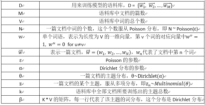
LDA概率模型

\[P({\boldsymbol {W}},{\boldsymbol {Z}},{\boldsymbol {\theta }},{\boldsymbol {\varphi }};\alpha ,\beta )=\prod _{i=1}^{K}P(\varphi _{i};\beta )\prod _{j=1}^{M}P(\theta _{j};\alpha )\prod _{t=1}^{N}P(Z_{j,t}\mid \theta _{j})P(W_{j,t}\mid \varphi _{Z_{j,t}})\]

LDA概率模型推导过程

对\(\beta\),\(\varphi\)求二重积分

\[{\begin{aligned}&P({\boldsymbol {Z}},{\boldsymbol {W}};\alpha ,\beta )=\int _{\boldsymbol {\theta }}\int _{\boldsymbol {\varphi }}P({\boldsymbol {W}},{\boldsymbol {Z}},{\boldsymbol {\theta }},{\boldsymbol {\varphi }};\alpha ,\beta )\,d{\boldsymbol {\varphi }}\,d{\boldsymbol {\theta }}\\={}&\int _{\boldsymbol {\varphi }}\prod _{i=1}^{K}P(\varphi _{i};\beta )\prod _{j=1}^{M}\prod _{t=1}^{N}P(W_{j,t}\mid \varphi _{Z_{j,t}})\,d{\boldsymbol {\varphi }}\int _{\boldsymbol {\theta }}\prod _{j=1}^{M}P(\theta _{j};\alpha )\prod _{t=1}^{N}P(Z_{j,t}\mid \theta _{j})\,d{\boldsymbol {\theta }}.\end{aligned}}\]

对于\(\theta\),

\[\int _{\boldsymbol {\theta }}\prod _{j=1}^{M}P(\theta _{j};\alpha )\prod _{t=1}^{N}P(Z_{j,t}\mid \theta _{j})\,d{\boldsymbol {\theta }}=\prod _{j=1}^{M}\int _{\theta _{j}}P(\theta _{j};\alpha )\prod _{t=1}^{N}P(Z_{j,t}\mid \theta _{j})\,d\theta_{j}\]

其中, \(\theta \sim {Dir}(\alpha)\),所以

\[\int _{\theta _{j}}P(\theta _{j};\alpha )\prod _{t=1}^{N}P(Z_{j,t}\mid \theta _{j})\,d\theta _{j}=\int _{\theta _{j}}{\frac {\Gamma \left(\sum _{i=1}^{K}\alpha _{i}\right)}{\prod _{i=1}^{K}\Gamma (\alpha _{i})}}\prod _{i=1}^{K}\theta _{j,i}^{\alpha _{i}-1}\prod _{t=1}^{N}P(Z_{j,t}\mid \theta _{j})\,d\theta_{j}\]

对于 \(\prod_{t=1}^{N}P(Z_{j,t}\mid\theta_{j})\),

\[\prod _{t=1}^{N}P(Z_{j,t}\mid \theta _{j})=\prod _{i=1}^{K}\theta _{j,i}^{n_{j,(\cdot )}^{i}}\]

首先因为\(z_{i,j}\sim \operatorname {Multinomial} (\theta _{i})\) 其中\(n_{j,r}^{i}\)表示第\(j^{th}\)篇文档中作为第\(i^{th}\)个主题的在词汇表中的第\(r^{th}\)个单词出现的次数。所以，\(n_{j,r^{i}}\)是三维的。如果三维中的任何一个维度不受特定值的限制，我们使用带圆括号的点\((\cdot)\)来表示。例如，\(n_{j,(\cdot)}^{i}\)表示在\(j^{th}\)文档中所有作为第\(i^{th}\)个主题的所有单词出现次数

所以对于\(\theta_{j}\)的积分可以转换成

\[\int _{\theta _{j}}{\frac {\Gamma \left(\sum _{i=1}^{K}\alpha _{i}\right)}{\prod _{i=1}^{K}\Gamma (\alpha _{i})}}\prod _{i=1}^{K}\theta _{j,i}^{\alpha _{i}-1}\prod _{i=1}^{K}\theta _{j,i}^{n_{j,(\cdot )}^{i}}\,d\theta _{j}=\int _{\theta _{j}}{\frac {\Gamma \left(\sum _{i=1}^{K}\alpha _{i}\right)}{\prod _{i=1}^{K}\Gamma (\alpha _{i})}}\prod _{i=1}^{K}\theta _{j,i}^{n_{j,(\cdot )}^{i}+\alpha_{i}-1}\,d\theta_{j}\]

又因为 \(\int_{\theta _{j}}{\frac {\Gamma \left(\sum _{i=1}^{K}n_{j,(\cdot )}^{i}+\alpha _{i}\right)}{\prod _{i=1}^{K}\Gamma (n_{j,(\cdot )}^{i}+\alpha _{i})}}\prod _{i=1}^{K}\theta _{j,i}^{n_{j,(\cdot )}^{i}+\alpha _{i}-1}\,d\theta_{j}=1\)

所以 \({\begin{aligned}&\int _{\theta _{j}}P(\theta _{j};\alpha )\prod _{t=1}^{N}P(Z_{j,t}\mid \theta _{j})\,d\theta _{j}=\int _{\theta _{j}}{\frac {\Gamma \left(\sum _{i=1}^{K}\alpha _{i}\right)}{\prod _{i=1}^{K}\Gamma (\alpha _{i})}}\prod _{i=1}^{K}\theta _{j,i}^{n_{j,(\cdot )}^{i}+\alpha _{i}-1}\,d\theta _{j}\\[8pt]={}&{\frac {\Gamma \left(\sum _{i=1}^{K}\alpha _{i}\right)}{\prod _{i=1}^{K}\Gamma (\alpha _{i})}}{\frac {\prod _{i=1}^{K}\Gamma (n_{j,(\cdot )}^{i}+\alpha _{i})}{\Gamma \left(\sum _{i=1}^{K}n_{j,(\cdot )}^{i}+\alpha _{i}\right)}}\int _{\theta _{j}}{\frac {\Gamma \left(\sum _{i=1}^{K}n_{j,(\cdot )}^{i}+\alpha _{i}\right)}{\prod _{i=1}^{K}\Gamma (n_{j,(\cdot )}^{i}+\alpha _{i})}}\prod _{i=1}^{K}\theta _{j,i}^{n_{j,(\cdot )}^{i}+\alpha _{i}-1}\,d\theta _{j}\\[8pt]={}&{\frac {\Gamma \left(\sum _{i=1}^{K}\alpha _{i}\right)}{\prod _{i=1}^{K}\Gamma (\alpha _{i})}}{\frac {\prod _{i=1}^{K}\Gamma (n_{j,(\cdot )}^{i}+\alpha _{i})}{\Gamma \left(\sum _{i=1}^{K}n_{j,(\cdot )}^{i}+\alpha_{i}\right)}}.\end{aligned}}\)

对于\(\varphi\), 跟\(\theta\)相同的过程

\[{\begin{aligned}&\int _{\boldsymbol {\varphi }}\prod _{i=1}^{K}P(\varphi _{i};\beta )\prod _{j=1}^{M}\prod _{t=1}^{N}P(W_{j,t}\mid \varphi _{Z_{j,t}})\,d{\boldsymbol {\varphi }}\\[8pt]={}&\prod _{i=1}^{K}\int _{\varphi _{i}}P(\varphi _{i};\beta )\prod _{j=1}^{M}\prod _{t=1}^{N}P(W_{j,t}\mid \varphi _{Z_{j,t}})\,d\varphi _{i}\\[8pt]={}&\prod _{i=1}^{K}\int _{\varphi _{i}}{\frac {\Gamma \left(\sum _{r=1}^{V}\beta _{r}\right)}{\prod _{r=1}^{V}\Gamma (\beta _{r})}}\prod _{r=1}^{V}\varphi _{i,r}^{\beta _{r}-1}\prod _{r=1}^{V}\varphi _{i,r}^{n_{(\cdot ),r}^{i}}\,d\varphi _{i}\\[8pt]={}&\prod _{i=1}^{K}\int _{\varphi _{i}}{\frac {\Gamma \left(\sum _{r=1}^{V}\beta _{r}\right)}{\prod _{r=1}^{V}\Gamma (\beta _{r})}}\prod _{r=1}^{V}\varphi _{i,r}^{n_{(\cdot ),r}^{i}+\beta _{r}-1}\,d\varphi _{i}\\[8pt]={}&\prod _{i=1}^{K}{\frac {\Gamma \left(\sum _{r=1}^{V}\beta _{r}\right)}{\prod _{r=1}^{V}\Gamma (\beta _{r})}}{\frac {\prod _{r=1}^{V}\Gamma (n_{(\cdot ),r}^{i}+\beta _{r})}{\Gamma \left(\sum _{r=1}^{V}n_{(\cdot ),r}^{i}+\beta_{r}\right)}}.\end{aligned}}\]

最终它们的双重积分等于

\[P({\boldsymbol {Z}},{\boldsymbol {W}};\alpha ,\beta )=\prod _{j=1}^{M}{\frac {\Gamma \left(\sum _{i=1}^{K}\alpha _{i}\right)}{\prod _{i=1}^{K}\Gamma (\alpha _{i})}}{\frac {\prod _{i=1}^{K}\Gamma (n_{j,(\cdot )}^{i}+\alpha _{i})}{\Gamma \left(\sum _{i=1}^{K}n_{j,(\cdot )}^{i}+\alpha _{i}\right)}}\times \prod _{i=1}^{K}{\frac {\Gamma \left(\sum _{r=1}^{V}\beta _{r}\right)}{\prod _{r=1}^{V}\Gamma (\beta _{r})}}{\frac {\prod _{r=1}^{V}\Gamma (n_{(\cdot ),r}^{i}+\beta _{r})}{\Gamma \left(\sum _{r=1}^{V}n_{(\cdot ),r}^{i}+\beta_{r}\right)}}\]

未完待续…