The Fundamentals of SVM
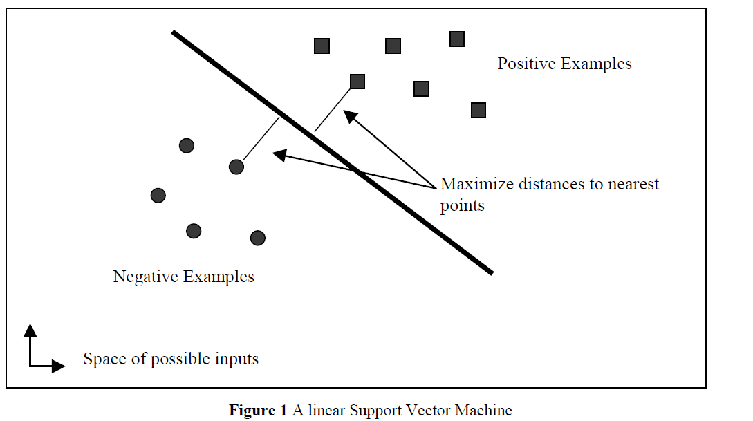
In the Machine Learing, the support vector machine is a model algorithm that defines which category an element belongs to.
We could define a hyperplane which is \(u = \vec{w}\cdot \vec{x} - b\) (or \(u = \vec{w}\cdot \vec{x} + b\)), the plane has N - 1 dimensions if the sample space is N dimensions.
We define the margin of 2 hyperplanes between these 2 classes to classfiy them if this datas’ u is bigger than 1 or less than -1 , so the margin of these 2 hyperplanes \(\vec{w}\cdot \vec{x_i} - b = 1\) and \(\vec{w}\cdot \vec{x_i} - b = -1\) is
\[d = \frac {2}{||\vec{w}||}\]The support vector machine is doing in the optimization objective is it’s minimizing the squared norm of the square length of the parameter vector \(\vec{w}\)
Application
-
Classification of images
-
Recognize the hand-written characters
SVM Decison Boundary
\(\min_{\vec{w},b} \frac {1}{2}||\vec{w}||^{2}\) subject to \(y_{i}(\vec{w}\cdot \vec{x_i} + b ) \geq 1, \forall {i}\)
For the extremum problem of convex function, we need to refer to a method, Lagrange Multiplier Method
Lagrange Multiplier
L(x, y, λ) = ƒ(x,y) + λ(φ(x,y) - c) = 0
=> \(L(w, b, \lambda) = \frac {1}{2}w^Tw + \sum_{i = 1}^{N}\lambda_i(1 - y_i(w^Tx_i + b))\)
Accoding to strong duality property,
\(\min_{w, b}\max_{\lambda}L(w, b, \lambda) = \min_{\lambda}\max_{w, b}L(w, b, \lambda)\)
subject to \(\lambda_i \geq 0\)
The partial derivatives of L equal to 0
\[\frac {\partial L}{\partial b} = 0 => \sum_{i = 1}^{N}\lambda_iy_i = 0\]\(\begin{aligned}L(w,b,\lambda)&=\frac {1}{2}w^Tw + \sum_{i = 1}^{N}\lambda_i - \sum_{i = 1}^{N}\lambda_iy_i(w^Tx_i + b)\\&=\frac {1}{2}w^Tw + \sum_{i = 1}^{N}\lambda_i - \sum_{i = 1}^{N}\lambda_iy_iw^Tx_i\end{aligned}\) where \(\sum_{i = 1}^{N}\lambda_iy_i = 0\)
\[\begin{aligned}\frac {\partial L}{\partial w} &= 0 \\\frac {\partial (\frac {1}{2}w^Tw + \sum_{i = 1}^{N}\lambda_i - \sum_{i = 1}^{N}\lambda_iy_iw^Tx_i)}{\partial w}&= 0\\\frac {1}{2}\cdot2w - \sum_{i = 1}^{N}\lambda_iy_ix_i &= 0\\w - \sum_{i = 1}^{N}\lambda_iy_ix_i &= 0\\=>w &= \sum_{i = 1}^{N}\lambda_iy_ix_i\end{aligned}\] \[\begin{aligned}L(w, b, \lambda) &= \frac {1}{2}(\sum_{i = 1}^{N}\lambda_iy_ix_i)^T(\sum_{j = 1}^{N}\lambda_jy_jx_j) + \sum_{i = 1}^{N}\lambda_i(1 - y_i(\sum_{i = 1}^{N}\lambda_jy_jx_j)^Tx_i + b)\\ &=\frac {1}{2}\sum_{i = 1}^{N}\sum_{j = 1}^{N}\lambda_i\lambda_jy_iy_jx_i^Tx_j + \sum_{i = 1}^{N}\lambda_i - \sum_{i = 1}^{N}\sum_{j = 1}^{N}\lambda_i\lambda_jy_iy_jx_j^Tx_i + 0\\&= -\frac {1}{2}\sum_{i = 1}^{N}\sum_{j = 1}^{N}\lambda_i\lambda_jy_iy_jx_i^Tx_j + \sum_{i = 1}^{N}\lambda_i \\&\forall i, \lambda_i \geq 0, \sum_{i = 1}^{N}\lambda_iy_i = 0\end{aligned}\]<=> \(\min_{\lambda} \frac {1}{2}\sum_{i = 1}^{N}\sum_{j = 1}^{N}\lambda_i\lambda_jy_iy_jx_i^Tx_j - \sum_{i = 1}^{N}\lambda_i \\\forall i, \lambda_i \geq 0, \sum_{i = 1}^{N}\lambda_iy_i = 0\)
KKT conditions
For solve a nonlinear optimization problem,
Optimize f(x) where subject to \(g_j(x) \leq 0(j = 1,...,m), \\h_k(x) = 0(k = 1,...,l)\), x is belongs to X , we could use the Lagrange function \(L(\mathbf{x}, \mu, \lambda) = f(x) + \mu^Tg(\mathbf{x}) + \lambda^Th(\mathbf{x})\)
where \(g(\mathbf{x}) = (g_1(\mathbf{x})), ...,(g_m(\mathbf{x}))^T, h(\mathbf{x}) = (h_1(\mathbf{x})), ...,(h_l(\mathbf{x}))^T\)
The KKT conditions to judge whether x is the optimize result is
\[\left\{\begin{array}{l} \frac{\partial f}{\partial x_i} + \sum\limits_{j = 1}^m\mu_j \frac{\partial g_j}{\partial x_i} + \sum\limits_{k = 1}^l \lambda_k\frac{\partial h_k}{\partial x_i} = 0,\rm{ }\left( {i = 1,2,...,n} \right)\\ h_k\left(\bf{x} \right) = 0,\rm{ (}k = 1,2, \cdots ,l)\\ {\mu_j}{g_j}\left(\bf{x} \right) = 0,\rm{ (}j = 1,2, \cdots ,m)\\ {\mu_j} \ge 0. \end{array} \right.\]due to our svm problem is a convex quadratic programming problem,
\[\begin{aligned}\exists (x_k, y_k), 1-y_k(wx_k + b) = 0 =>y_k(wx_k + b) &= 1\\y_k^2(wx_k + b) &= y_k\\wx_k + b &= y_k(\because y_k^2 = 1)\\b &= y_k - \sum_{j = 1}^{N}\lambda_iy_ix_i^Tx_k\end{aligned}\]We got the equation of w and b , which could be solved by training dataset to get the λ then calculate them
Soft-margin
Because not all datas are linearly separable, we should introduce the error margin which is built by hinge loss function, \(\zeta_i = max(0, 1 - y_i(\vec{w}\cdot \vec{x_i} + b))\)
\[\min_\vec{w} \frac {1}{2}||\vec{w}||^{2} => \min_{w}\frac {1}{2}w^Tw +C\sum_{i=0}^N\zeta_i\]subject to \(y_{i}(\vec{w}\cdot \vec{x_i} + b ) \geq 1 - \zeta_i, \zeta_i \geq 0,\forall {i}\)
Let’s complute again
1.Introduce Lagrange function
\[L(\vec{w}, b, \zeta_i, \lambda, \beta) = \frac{1}{2}||\vec{w}||^2 + C \cdot \sum_{i = 1}^N\zeta_i + \sum_{i = 1}^N\lambda_i(1 - \zeta_i - y_i(\vec{w} \cdot \vec{x_i} + b))+\sum_{i = 1}^N\beta_i(-\zeta_i)\]2.The partial derivative of Lagrange function
\[\left\{\begin{matrix} \frac {\partial L}{\partial \vec{w}}=0=>\vec{w}-\sum_{i = 1}^N\lambda_iy_i\vec{x_i} =0=>\vec{w}=\sum_{i = 1}^N\lambda_iy_i\vec{x_i}\\ \frac {\partial L}{\partial b}=0=>\sum_{i = 1}^N\lambda_iy_i=0\\ \frac {\partial L}{\partial \zeta_i}=0=>C-\lambda_i-\beta_i=0=>C = \lambda_i+\beta_i \end{matrix}\right.\] \[\begin{aligned} L(\vec{w}, b, \zeta_i, \lambda, \beta)_{min} &= \frac{1}{2}||\vec{w}||^2 + C \cdot \sum_{i = 1}^N\zeta_i + \sum_{i = 1}^N\lambda_i(1 - \zeta_i - y_i(\vec{w} \cdot \vec{x_i} + b))+\sum_{i = 1}^N\beta_i(-\zeta_i)\\&=\frac{1}{2}||\vec{w}||^2 + C \cdot \sum_{i = 1}^N\zeta_i + \sum_{i = 1}^N\lambda_i - \sum_{i = 1}^N\lambda_i\zeta_i- \sum_{i = 1}^N\lambda_iy_i\vec{w} \cdot \vec{x_i}+\sum_{i = 1}^N\lambda_iy_ib-\sum_{i = 1}^N\beta_i\zeta_i\\&=\frac{1}{2}(\sum_{i = 1}^N\lambda_iy_i\vec{x_i})^2+(\lambda_i+\beta_i)\sum_{i = 1}^N\zeta_i+\sum_{i = 1}^N\lambda_i-\sum_{i = 1}^N\lambda_i\zeta_i-\sum_{i = 1}^N\lambda_iy_i(\sum_{j = 1}^N\lambda_jy_j\vec{x_j})\cdot \vec{x_i}+0-\sum_{i = 1}^N\beta_i\zeta_i\\&=\frac{1}{2}\sum_{i = 1}^N\lambda_i\lambda_jy_iy_j\vec{x_i}\vec{x_j}+\sum_{i = 1}^N\lambda_i\zeta_i+\sum_{i = 1}^N\beta_i\zeta_i+\sum_{i = 1}^N\lambda_i-\sum_{i = 1}^N\lambda_i\zeta_i-\sum_{i = 1}^N\lambda_i\lambda_jy_iy_j\vec{x_i}\vec{x_j}-\sum_{i = 1}^N\beta_i\zeta_i\\=&-\frac{1}{2}\sum_{i = 1}^N\lambda_i\lambda_jy_iy_j\vec{x_i}\vec{x_j}+\sum_{i = 1}^N\lambda_i\end{aligned}\]3.Strong duality property
\(\min_{w, b}\max_{\lambda}L(w, b, \lambda) = \min_{\lambda}\max_{w, b}L(w, b, \lambda)\)
subject to \(\lambda_i \geq 0\)
4.KKT conditions
\[\left\{\begin{array}{l} \frac{\partial f}{\partial x_i} + \sum\limits_{j = 1}^m\mu_j \frac{\partial g_j}{\partial x_i} + \sum\limits_{k = 1}^l \lambda_k\frac{\partial h_k}{\partial x_i} = 0,\rm{ }\left( {i = 1,2,...,n} \right)\\ h_k\left(\bf{x} \right) = 0,\rm{ (}k = 1,2, \cdots ,l)\\ {\mu_j}{g_j}\left(\bf{x} \right) = 0,\rm{ (}j = 1,2, \cdots ,m)\\ {\mu_j} \ge 0. \end{array} \right.\] \[\Rightarrow \left\{\begin{matrix} \mu g(\vec{x}) = \begin{bmatrix} \sum_{i = 1}^N\lambda_i(1 - \zeta_i - y_i(\vec{w} \cdot \vec{x_i} + b)) & \sum_{i = 1}^N\beta_i(-\zeta_i) \end{bmatrix}=0\\ g(x)=\begin{bmatrix}\sum_{i = 1}^N(1 - \zeta_i - y_i(\vec{w} \cdot \vec{x_i} + b)) & \sum_{i = 1}^N-\zeta_i\end{bmatrix} \leq 0\\ \mu = \begin{bmatrix} \lambda& \beta \end{bmatrix}\geq 0 \end{matrix}\right.\] \[\left\{\begin{matrix} min_{\lambda}max_{\vec{w},b}L(\vec{w}, b, \zeta_i, \lambda, \beta) = \frac{1}{2}\sum_{i = 1}^N\lambda_i\lambda_jy_iy_j\vec{x_i}\vec{x_j}-\sum_{i = 1}^N\lambda_i\\ s.t.\sum_{i = 1}^N\lambda_iy_i=0\\ C-\lambda_i-\beta_i=0\\ \lambda_i\geq 0\\ \beta_i\geq 0 \end{matrix}\right.\] \[\left.\begin{matrix} C-\lambda_i-\beta_i=0\\ \lambda_i\geq 0\\ \beta_i\geq 0 \end{matrix}\right\}\Rightarrow 0\leqslant \lambda_i\leqslant C\] \[\begin{aligned}b^* &= y_i - \vec{w}\cdot \vec{x_i}\\&=y_i - \sum_{i = 1}^N\lambda_jy_j\vec{x_j}\vec{x_i} \end{aligned}\]5.Got result
\[\left\{\begin{matrix} \begin{aligned} \min_{\mathbf \lambda}{\frac{1}{2}\sum_{i=1}^{N}{\sum_{j=1}^{N}{y_iy_jK\left( \vec{x_i},\vec{x_j}\right)\lambda_i\lambda_j}}-\sum_{j=1}^{N}{\lambda_i}}\\ s.t. \ \ 0 \leq \lambda_i \leq C, \ i=1,\ldots,N \\ \sum_{i=1}^{N}{y_i \lambda_i} = 0\end{aligned} \end{matrix}\right.\Leftrightarrow \left\{\begin{matrix} \begin{aligned} \min_\mathbf{\lambda}{\frac{1}{2}\mathbf{\lambda^T Q \lambda} -\mathbf{1^T\lambda}}\\ s.t. \ \ \ \mathbf 0 \preceq \mathbf \lambda \preceq C\cdot \mathbf 1 \\ \mathbf {\lambda^T y} = 0 \end{aligned} \end{matrix}\right.\]Q is symmetric matrix and \(\mathbf {Q_{ij}} = y_i y_j K\left( \mathbf{x_i}, \mathbf{x_j} \right)\)
You could found that \(\mathbf{\lambda^T Q \lambda} \geq 0\) shows L is convex function , and Q is positive semi-definite , \(K( \mathbf{x_i}, \mathbf{x_j})\) must be a positive definte matrix
Kernel methods
The dot product of \(\vec{x_i}\cdot \vec{x_j}\) could be replaced by a nonlinear kernel function. If the dataset is nonlinear separable speraly, the kernel trick may be took into low dimensional space to high dimensional space
Linear Kernel
\[K(x, {x}') = {x}'^{T}x\]RBF Kernel
\[K(x, {x}') = exp(- \frac {||x-{x}'||^2_2}{2\sigma^2})\]\(\left \| x-{x}' \right \|_{2}^{2}\) is squre of euclidean distance
Exponential Kernel
\[K(x, {x}') = exp(- \frac {||x - {x}'||}{2\sigma^2})\]Laplacian Kernel
\[K(x, {x}') = exp(- \frac {||x - {x}'||}{\sigma})\]Polynomial Kernel
\[K(x, {x}') = ({x}'^{T}x + c)^d\]The d is float , optional, and default=3
Sigmoid Kernel
\[K(x, {x}') = tanh(\alpha x^{T}{x}' + c)\]Log Kernel
\[K(x, {x}') = -log(1 + ||x - {x}')^d\]It usullay uses in image segmentation
Cauchy Kernel
\[K(x, {x}') = \frac {1}{1 + \frac {||x - {x}'||^{2}}{\sigma}}\]Bayesian Kernel
\[K(x, {x}') = \prod_{i=1}^N \kappa_i (x_i,{x}'_i)\]where \(\kappa_i(a,b) = \sum_{c \in \{0;1\}} P(Y=c \mid X_i=a) ~ P(Y=c \mid X_i=b)\)
Generalized T-Student Kernel
\[K(x, {x}') = \frac {1}{1 + ||x - {x}'||^d}\]SMO Algorithm
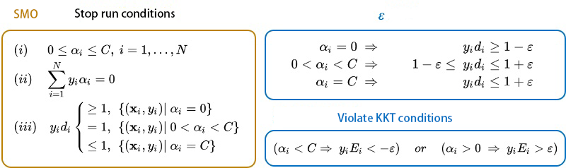
the α is λ
\[d_i=\sum_{j=1}^{N}{y_j \lambda_j k_{ji}} + b\]Sequential minimal optimization algorithm’s main idea is the sample size of each optimization is 2, update the λ and the Lagrange multiplier method is updated by heuristic method in each step
The main loop of this algorithm:
1.Calculate the error of predict value and real-value
\[E_i = f(x_i) - y_i = \sum_{j = 1}^N\lambda_jy_jK(\vec{x_i},\vec{x_j}) + b) - y_i\]2.Heuristic search the j which is max|Ej - Ei|
3.Complute the L and H, if L == H, exit loop
\[\left\{\begin{matrix} L = max(0, \lambda_j^{old}-\lambda_i^{old}), \ H = min(C, C + \lambda_j^{old}-\lambda_i^{old}) \ if \ y_i \neq y_j\\ L = max(0, \lambda_j^{old}+\lambda_i^{old}-C), \ H = min(C, \lambda_j^{old}+\lambda_i^{old}) \ if \ y_i = y_j \end{matrix}\right.\]4.Compute \(\eta\), if \(\eta \geq 0\), exit loop
\[\eta = 2K(\vec{x_i},\vec{x_j}) - K(\vec{x_i},\vec{x_j}) -K(\vec{x_i},\vec{x_j})\]5.Update \(\lambda_j\)
\[\lambda_j^{new} = \lambda_j^{old} + \frac {y_i(E_i - E_j)}{\eta}\]6.Clip the \(\lambda_j\)
\[\lambda_j^{new, clipped} = \left\{\begin{matrix} H \ \ \ \ \ \ \ \ if \ \lambda_j^{new} > H\\ \lambda_j^{new} \ \ \ \ \ \ \ \ \ \ if \ H \leq \lambda_j^{new} \leq L\\ L \ \ \ \ \ \ \ \ if \ \lambda_j^{new} < L \end{matrix}\right.\]7.Update \(\lambda_i\), we get 2 new \(\lambda\)
\[\lambda_i^{new} = \lambda_i^{old} + y_iy_j(\lambda_j^{old} - \lambda_j^{new, clipped})\]8.Calculate b1 and b2 to update b
\[\left\{\begin{matrix} b_1 = b^{old} - E_i - y_i(\lambda_i^{new} - \lambda_i^{old})K(\vec{x_i},\vec{x_i}) - y_j(\lambda_j^{new} - \lambda_j^{old})K(\vec{x_i},\vec{x_j})\\\ b_2 = b^{old} - E_j - y_i(\lambda_i^{new} - \lambda_i^{old})K(\vec{x_i},\vec{x_j}) - y_j(\lambda_j^{new} - \lambda_j^{old})K(\vec{x_j},\vec{x_j}) \end{matrix}\right.\\\Rightarrow b =\left\{\begin{matrix} b_1 \ \ \ \ \ \ \ \ \ \ \ \ \ 0 < \lambda_i^{new} < C\\\ b_2 \ \ \ \ \ \ \ \ \ \ \ \ \ 0 < \lambda_j^{new} < C\\ \frac{b_1+b_2}{2}\ \ \ \ \ \ \ other \end{matrix}\right.\]Pseudo code
target = desired output vector
point = training point matrix
procedure takeStep(i1,i2)
    if (i1 == i2) return 0
    alph1 = Lagrange multiplier for i1
    y1 = target[i1]
    E1 = SVM output on point[i1] – y1 (check in error cache)
    s = y1*y2
    Compute L, H via equations (13) and (14)
    if (L == H)
        return 0
    k11 = kernel(point[i1],point[i1])
    k12 = kernel(point[i1],point[i2])
    k22 = kernel(point[i2],point[i2])
    eta = k11+k22-2*k12
    if (eta > 0)
    {
        a2 = alph2 + y2*(E1-E2)/eta
        if (a2 < L) a2 = L
        else if (a2 > H) a2 = H
    }
    else
    {
        Lobj = objective function at a2=L
        Hobj = objective function at a2=H
        if (Lobj < Hobj-eps)
            a2 = L
        else if (Lobj > Hobj+eps)
            a2 = H
        else
            a2 = alph2
    }
    if (|a2-alph2| < eps*(a2+alph2+eps))
        return 0
    a1 = alph1+s*(alph2-a2)
    Update threshold to reflect change in Lagrange multipliers
    Update weight vector to reflect change in a1 & a2, if SVM is linear
    Update error cache using new Lagrange multipliers
    Store a1 in the alpha array
    Store a2 in the alpha array
    return 1
endprocedure

procedure examineExample(i2)
    y2 = target[i2]
    alph2 = Lagrange multiplier for i2
    E2 = SVM output on point[i2] – y2 (check in error cache)
    r2 = E2*y2
    if ((r2 < -tol && alph2 < C) || (r2 > tol && alph2 > 0))
    {
        if (number of non-zero & non-C alpha > 1)
        {
            i1 = result of second choice heuristic (section 2.2)
            if takeStep(i1,i2)
                return 1
        }
        loop over all non-zero and non-C alpha, starting at a random point
        {
            i1 = identity of current alpha
            if takeStep(i1,i2)
                return 1
        }
        loop over all possible i1, starting at a random point
        {
            i1 = loop variable
            if (takeStep(i1,i2)
                return 1
        }
    }
    return 0
endprocedure

main routine:
    numChanged = 0;
    examineAll = 1;
    while (numChanged > 0 | examineAll)
    {
        numChanged = 0;
        if (examineAll)
            loop I over all training examples
            numChanged += examineExample(I)
        else
            loop I over examples where alpha is not 0 & not C
            numChanged += examineExample(I)
        if (examineAll == 1)
            examineAll = 0
        else if (numChanged == 0)
            examineAll = 1
    }
The classifiers comparison
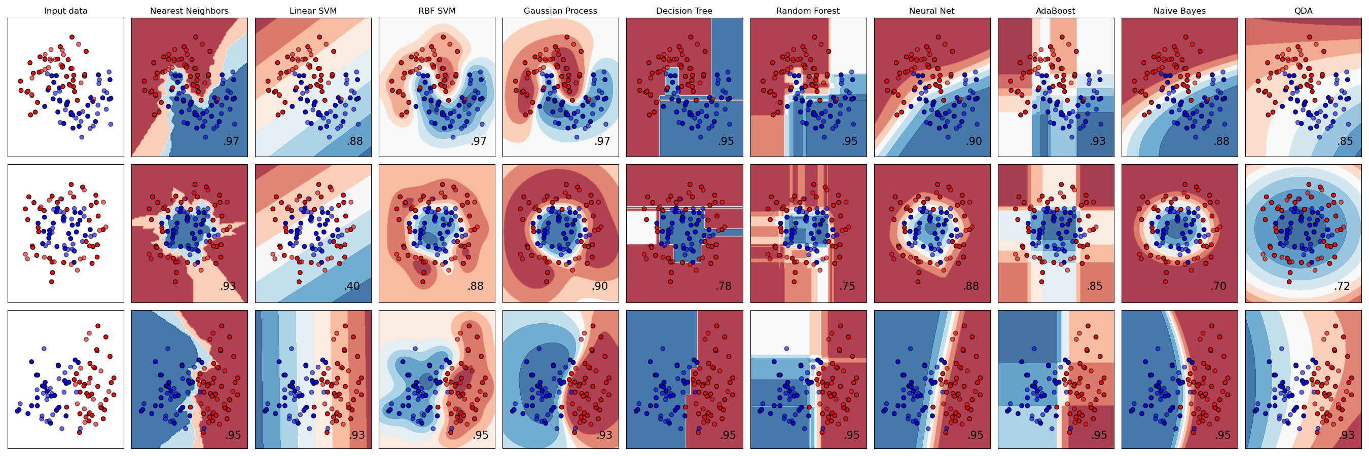
Content
import numpy as np
import matplotlib.pyplot as plt
from matplotlib.colors import ListedColormap
from sklearn.model_selection import train_test_split
from sklearn.preprocessing import StandardScaler
from sklearn.datasets import make_moons, make_circles, make_classification
from sklearn.neural_network import MLPClassifier
from sklearn.neighbors import KNeighborsClassifier
from sklearn.svm import SVC
from sklearn.gaussian_process import GaussianProcessClassifier
from sklearn.gaussian_process.kernels import RBF
from sklearn.tree import DecisionTreeClassifier
from sklearn.ensemble import RandomForestClassifier, AdaBoostClassifier
from sklearn.naive_bayes import GaussianNB
from sklearn.discriminant_analysis import QuadraticDiscriminantAnalysis

h = .02  # step size in the mesh

names = ["Nearest Neighbors", "Linear SVM", "RBF SVM", "Gaussian Process",
         "Decision Tree", "Random Forest", "Neural Net", "AdaBoost",
         "Naive Bayes", "QDA"]

classifiers = [
    KNeighborsClassifier(3),
    SVC(kernel="linear", C=0.025),
    SVC(gamma=2, C=1),
    GaussianProcessClassifier(1.0 * RBF(1.0)),
    DecisionTreeClassifier(max_depth=5),
    RandomForestClassifier(max_depth=5, n_estimators=10, max_features=1),
    MLPClassifier(alpha=1, max_iter=1000),
    AdaBoostClassifier(),
    GaussianNB(),
    QuadraticDiscriminantAnalysis()]

X, y = make_classification(n_features=2, n_redundant=0, n_informative=2,
                           random_state=1, n_clusters_per_class=1)
rng = np.random.RandomState(2)
X += 2 * rng.uniform(size=X.shape)
linearly_separable = (X, y)

datasets = [make_moons(noise=0.3, random_state=0),
            make_circles(noise=0.2, factor=0.5, random_state=1),
            linearly_separable
            ]

figure = plt.figure(figsize=(27, 9))
i = 1
# iterate over datasets
for ds_cnt, ds in enumerate(datasets):
    # preprocess dataset, split into training and test part
    X, y = ds
    X = StandardScaler().fit_transform(X)
    X_train, X_test, y_train, y_test = \
        train_test_split(X, y, test_size=.4, random_state=42)

    x_min, x_max = X[:, 0].min() - .5, X[:, 0].max() + .5
    y_min, y_max = X[:, 1].min() - .5, X[:, 1].max() + .5
    xx, yy = np.meshgrid(np.arange(x_min, x_max, h),
                         np.arange(y_min, y_max, h))

    # just plot the dataset first
    cm = plt.cm.RdBu
    cm_bright = ListedColormap(['#FF0000', '#0000FF'])
    ax = plt.subplot(len(datasets), len(classifiers) + 1, i)
    if ds_cnt == 0:
        ax.set_title("Input data")
    # Plot the training points
    ax.scatter(X_train[:, 0], X_train[:, 1], c=y_train, cmap=cm_bright,
               edgecolors='k')
    # Plot the testing points
    ax.scatter(X_test[:, 0], X_test[:, 1], c=y_test, cmap=cm_bright, alpha=0.6,
               edgecolors='k')
    ax.set_xlim(xx.min(), xx.max())
    ax.set_ylim(yy.min(), yy.max())
    ax.set_xticks(())
    ax.set_yticks(())
    i += 1

    # iterate over classifiers
    for name, clf in zip(names, classifiers):
        ax = plt.subplot(len(datasets), len(classifiers) + 1, i)
        clf.fit(X_train, y_train)
        score = clf.score(X_test, y_test)

        # Plot the decision boundary. For that, we will assign a color to each
        # point in the mesh [x_min, x_max]x[y_min, y_max].
        if hasattr(clf, "decision_function"):
            Z = clf.decision_function(np.c_[xx.ravel(), yy.ravel()])
        else:
            Z = clf.predict_proba(np.c_[xx.ravel(), yy.ravel()])[:, 1]

        # Put the result into a color plot
        Z = Z.reshape(xx.shape)
        ax.contourf(xx, yy, Z, cmap=cm, alpha=.8)

        # Plot the training points
        ax.scatter(X_train[:, 0], X_train[:, 1], c=y_train, cmap=cm_bright,
                   edgecolors='k')
        # Plot the testing points
        ax.scatter(X_test[:, 0], X_test[:, 1], c=y_test, cmap=cm_bright,
                   edgecolors='k', alpha=0.6)

        ax.set_xlim(xx.min(), xx.max())
        ax.set_ylim(yy.min(), yy.max())
        ax.set_xticks(())
        ax.set_yticks(())
        if ds_cnt == 0:
            ax.set_title(name)
        ax.text(xx.max() - .3, yy.min() + .3, ('%.2f' % score).lstrip('0'),
                size=15, horizontalalignment='right')
        i += 1

plt.tight_layout()
plt.show()
Obviously, the RBF is best classifier, so how to choose the kernels is
-
If the train samples have large the features, please choose the linear kernel
-
If the samples have few of the features, you could choose RBF Kernel
-
If have lots of the samples but the features not, you could add some features by yourself, then choose the linear kernel.
Source code
#coding:utf-8
#Author: Toryun
#Date: 2020-07-09 18:09:00
import matplotlib.pyplot as plt
import numpy as np
from mpl_toolkits.mplot3d import Axes3D
from sklearn import svm #对比
from sklearn.datasets import load_digits
from sklearn.model_selection import train_test_split
from sklearn.metrics import classification_report
import pickle
import os
'''
http://jmlr.csail.mit.edu/papers/volume11/cawley10a/cawley10a.pdf
http://jmlr.csail.mit.edu/papers/volume8/cawley07a/cawley07a.pdf
libsvm源码论文http://www.csie.ntu.edu.tw/~cjlin/papers/libsvm.pdf
核函数选取的方法https://www.csie.ntu.edu.tw/~cjlin/papers/guide/guide.pdf
1. 如果特征的数量大到和样本数量差不多,则选用线性核
2. 如果特征的数量小,样本的数量正常,则选用高斯核函数
3. 如果特征的数量小,而样本的数量很大,则需要手工添加一些特征从而变成第一种情况
svm原论文中文翻译https://zhuanlan.zhihu.com/p/23068673
sklearn数据集文件地址: /Library/Frameworks/Python.framework/Versions/2.7/lib/python2.7/site-packages/sklearn/datasets/data
'''
__all__ = [
"loadData",
"Kernel",
"heurstic_selectJ",
"calEi",
"Normal_vector",
"SMOv1",
"SMOv2",
"innerLoop",
"show3DClassifer",
"predict",
"show2DData",
"cmp_sklearn_svm"
]
def loadData(filepath):
'''
加载数据并分类
return: 数据集和标签集
'''
datas = []
labels = []
f = open(filepath)
for i in f.readlines():
l = i.strip().split('\t')
datas.append((float(l[0]), float(l[1])))
labels.append(float(l[2]))
return datas, labels
def show2DData(datas, labels):
'''
function: 可视化样本数据
datas: list
labels: list
rtype: none
'''
data_positive = []
data_negetive = []
for i in range(len(datas)):
#分类
if labels[i] > 0:
data_positive.append(datas[i])
else:
data_negetive.append(datas[i])
x_p, y_p = np.transpose(np.array(data_positive))[0], np.transpose(np.array(data_positive))[1]
x_n, y_n = np.transpose(np.array(data_negetive))[0], np.transpose(np.array(data_negetive))[1]
plt.scatter(x_p, y_p)
plt.scatter(x_n, y_n)
plt.show()
class SVM(object):
'''
求最小间隔margin
1/2||w||^2
s.t. y_i(w^Tx_i + b)>= 1, i = 1,2,..,n
核心步骤
1. 计算误差Ei,Ej
2. 计算alpha上下界L,H
3. 计算学习速率theta = 2*K(xi, xj) - K(xi, xi) - K(xj, xj)
4. 更新alpha_i, 和alpha_j
5. 计算b1,b2, 并更新b
'''
def __init__(self, datas, labels, C, tol, maxIter, kwg):
self.X = np.mat(datas) #自变量X向量shape(m,n)
self.y = np.mat(labels).transpose() #(+1,-1)数据集shape(m, 1)
self.w = np.zeros((len(datas[0]), 1)) #超平面的法向量w
self.C = C #惩罚系数一般为1
self.tol = tol #误差上限一般为1e4 (Tolerance for stopping criteria) float, optional.
self.m = len(datas) #矩阵长度
self.K = np.mat(np.zeros((self.m, self.m)))
self.b = 0 #阈值
self.maxIter = maxIter #最大迭代次数
self.alphas = np.mat(np.zeros((self.m, 1))) #超参数由拉格朗日函数引入
self.eCache = np.mat(np.zeros((self.m, 2))) #存储误差Ei = Ui-yi
self.kwargs = kwg #核函数的选择linear, rbf, poly等
self.nonzeralphas_train = None #用于保存训练模型中的非0alpha下标
self.support_vector_X = None #训练过的支持向量
self.support_vector_alphas = None #支持向量参数alphas
self.support_vector_labels = None #支持向量标签
def Kernel(self, x1, x2):
'''
核函数:
线性核函数linear: x1*x2
多项式核函数poly: (x1*x2 + C)^d 可以使原来线性不可分的样本数据变为线性可分
高斯核函数rbf(Radial Basis Function Kernel) 正态分布E^{(||x1-x2||^2)/-2*theta^2}
拉普拉斯核函数Laplace
Sigmoid
具体参考sklearn svm源代码
'''
#初始化一个矩阵保存计算结果
KT = np.mat(np.zeros((self.m,1)))
if self.kwargs['kernel'] == 'linear':
return x1 * x2.T
elif self.kwargs['kernel'] == 'rbf':
#theta默认1.3
theta = self.kwargs['theta']
for j in range(self.m):
delta = x1[j,:] - x2
KT[j] = delta * delta.T
return np.exp(KT / (-2.0 * theta**2))
elif self.kwargs['kernel'] == 'poly':
KT = x1 * x2.T
degree = self.kwargs['degree'] #int, default=3
for j in range(self.m):
KT[j] = (KT[j] + self.C)**degree
return KT
elif self.kwargs['kernel'] == 'Laplace':
theta = self.kwargs['theta']
for j in range(self.m):
deltaX = x1[j,:] - x2
KT[j] = np.sqrt(deltaX * deltaX.T)
return np.exp( - KT / theta)
elif self.kwargs['kernel'] == 'sigmoid':
KT = x1 * x2.T
a = self.kwargs['a']
for j in range(self.m):
KT[j] = np.tanh(a * KT[j] + self.m)
else:
raise NameError("can't recognise the kernel mathod")
def calEi(self, i):
'''
计算误差Ei
Ei = ui - yi
'''
ui = float(np.multiply(self.alphas, self.y).T * self.K[:,i]) + self.b
Ei = ui - float(self.y[i])
return Ei
def heurstic_selectJ(self, i, Ei):
'''
启发式选择j,使得|Ej - Ei|最大
'''
maxK = -1
maxDeltaE = 0
Ej = 0
self.eCache[i] = [1, Ei] #更新,存入Ei
#查找误差Ei集合中的非0元素并返回所有下标
oneEcachelist = np.nonzero(self.eCache[:,0].A)[0]
if len(oneEcachelist) > 1:
for k in oneEcachelist:
if k == i:
continue
Ek = self.calEi(k)
deltaEk = abs(Ek - Ei)
if (deltaEk > maxDeltaE):
maxK = k
maxDeltaE = deltaEk
Ej = Ek
else:
maxK = i
while maxK == i:
maxK = np.random.choice(self.m)
Ej = self.calEi(maxK)
return maxK, Ej
def Normal_vector(self):
'''
计算w向量
datas: 数据矩阵
labels: (-1, +1)集合
alphas:
'''
#转换成array
for i in range(self.m):
self.w += np.multiply(self.alphas[i] * self.y[i], self.X[i, :].T)
def SMOv1(self):
'''
简化版smo算法,不包含启发式选择j参数
datas: 数据矩阵
labels: 标签(1, -1)
C: 松弛变量
tol: 容错率
maxIter: 最大迭代次数
b: 截距
alpha: 拉格朗日乘子
yi: +1, -1
xi: 数据集(向量)
w: 法向量 sum{alpha_i*yi*dataMats[i:]*dataMats^T}
fxi: sum{alpha_i*yi*xi^TxI} + b
Ei: 误差项Ei = fxi - yi
eta: 学习速率xi^Txi + xj^Txj - 2xi^Txj
数学公式:
min 1/2||w||^2
s.t. y_i(w^Tx_i + b)>= 1, i = 1,2,..,n
'''
for i in range(self.m):
self.K[:,i] = self.Kernel(self.X, self.X[i,:])
#初始化迭代次数
iternum = 0
#更新核矩阵
while (iternum < self.maxIter):
#统计alpha优化次数
alphachangenum = 0
for i in range(self.m):
#1. 计算误差Ei
yi = self.y[i]
Ei = self.calEi(i)
#优化alpha, 容错率
if((yi*Ei < -self.tol) and (self.alphas[i] < self.C)) or ((yi*Ei > self.tol) and (self.alphas[i] > 0)):
#随机选择alphaj并且不等于alphai
j = i
while j == i:
j = np.random.choice(self.m)
#计算误差Ej
yj = self.y[j]
Ej = self.calEi(j)
#保存更新前的alpha
alpha_i_old = self.alphas[i].copy()
alpha_j_old = self.alphas[j].copy()
#2. 计算alpha上下界
if yi != yj:#异侧
L = max(0, self.alphas[j] - self.alphas[i])
H = min(self.C, self.C + self.alphas[j] - self.alphas[i])
else: #同侧
L = max(0, self.alphas[j] + self.alphas[i] - self.C)
H = min(self.C, self.alphas[j] + self.alphas[i])
if L == H:
print("L == H")
continue
#3. 计算eta
eta = 2.0 * self.K[i,j] - self.K[i,i] - self.K[j,j]
if eta >= 0:#半正定
print("eta >= 0")
continue
#4. 更新alphaj
self.alphas[j] -= yj * (Ei - Ej)/eta
#5. 修剪alphaj
if self.alphas[j] > H:
self.alphas[j] = H
if self.alphas[j] < L:
self.alphas[j] = L
if abs(self.alphas[j] - alpha_j_old) < 0.00001:
print("alphas_{} = {} is updated".format(j, self.alphas[j]))
continue
#6. 更新alphai
s = yi*yj
self.alphas[i] += s*(alpha_j_old - self.alphas[j])
#7. 更新b1, b2
b1 = self.b - Ei - yi * (self.alphas[i] - alpha_i_old) * self.K[i,i] - yj * (self.alphas[j] - alpha_j_old) * self.K[i,j]
b2 = self.b - Ej - yi * (self.alphas[i] - alpha_i_old) * self.K[i,j] - yj * (self.alphas[j] - alpha_j_old) * self.K[j,j]
#8. 更新b
if 0 < self.alphas[i] and self.C > self.alphas[i]:
self.b = b1
elif 0 < self.alphas[j] and self.C > self.alphas[j]:
self.b = b2
else:
self.b = (b1 + b2) / 2.0
#更新优化统计
alphachangenum += 1
print("Iter:{} Smaples: No.{}, alphas update times:{}".format(iternum, i, alphachangenum))
if alphachangenum == 0:
iternum += 1
else:
iternum = 0
print("-----------------No.{}th iteration-----------------".format(iternum))
def SMOv2(self):
'''
完整版包含启发式选择j
datas: 数据矩阵
labels: 标签(1, -1)
C: 松弛变量
tol: 容错率
maxIter: 最大迭代次数
b: 截距
alpha: 拉格朗日乘子
yi: +1, -1
xi: 数据集(向量)
w: 法向量
fxi: sum{alpha_i*yi*xi^TxI} + b
Ei: 误差项Ei = fxi - yi
eta: 学习速率xi^Txi + xj^Txj - 2xi^Txj
数学公式:
min 1/2||w||^2
s.t. y_i(w^Tx_i + b)>= 1, i = 1,2,..,n
'''
#更新核矩阵
#迭代次数
iternum = 0
#遍历所有训练数据标识符
AllX = True
for i in range(self.m):
self.K[:,i] = self.Kernel(self.X, self.X[i,:])
#alpha更新次数
alphachangenum = 0
while (iternum < self.maxIter) and ((alphachangenum > 0) or (AllX)):
alphachangenum = 0
if AllX:
#遍历整个训练集
for i in range(self.m):
alphachangenum += self.innerLoop(i)
iternum += 1
else:
#遍历非边界子集(0<a<C),获取界内所有alpha下标的数组
nonBound = np.nonzero((self.alphas.A > 0) * (self.alphas.A < self.C))[0]
for i in nonBound:
alphachangenum += self.innerLoop(i)
iternum += 1
#交替
if AllX:
AllX = False
elif alphachangenum == 0:
#如果非边界的点没有更新alpha, 切换为遍历整个训练集
AllX = True
self.nonzeralphas_train = np.nonzero(self.alphas.A)[0]
self.support_vector_X = self.X[self.nonzeralphas_train]
self.support_vector_alphas = self.alphas[self.nonzeralphas_train]
self.support_vector_labels = self.y[self.nonzeralphas_train]
self.Normal_vector()
def innerLoop(self, i):
'''
找出不满足KKT条件的alpha,并优化
核心步骤:
1. 计算误差Ei,Ej
2. 计算alpha上下界L,H
3. 计算学习速率theta = 2*K(xi, xj) - K(xi, xi) - K(xj, xj)
4. 更新alpha_i, 和alpha_j
5. 计算b1,b2, 并更新b
退出循环条件: L == H, eta >= 0, alpha_j变化值很小等
'''
#1. 计算误差Ej
Ei = self.calEi(i)
yi = self.y[i]
if (yi*Ei < - self.tol and self.alphas[i] < self.C) or (yi * Ei > self.tol and self.alphas[i] > 0):
#1. 计算误差Ej
j, Ej = self.heurstic_selectJ(i, Ei)
yj = self.y[j]
#保存旧的alpha
alpha_i_old = self.alphas[i].copy()
alpha_j_old = self.alphas[j].copy()
#2. 计算alpha上下界
if yi != yj:
L = max(0, self.alphas[j] - self.alphas[i])
H = min(self.C, self.C + self.alphas[j] - self.alphas[i])
else:
L = max(0, self.alphas[j] + self.alphas[i] - self.C)
H = min(self.C, self.alphas[i] + self.alphas[j])
if L == H:
return 0
#3. 计算theta
eta = 2.0 * self.K[i,j] - self.K[i,i] - self.K[j,j]
if eta >= 0:
return 0
#4. 更新alpha_j
self.alphas[j] -= yj * (Ei - Ej) / eta
#修正alpha_j
if self.alphas[j] > H:
self.alphas[j] = H
if self.alphas[j] < L:
self.alphas[j] = L
#更新误差缓存Ej,1表示Ej被计算过
self.eCache[j] = [1, self.calEi(j)]
#如果alpha收敛到一定值,则退出(ε一般默认0.00001
if abs(alpha_j_old - self.alphas[j]) < 0.00001:
return 0
#4. 否则更新alpha_i
s = yj * yi
self.alphas[i] += s * (alpha_j_old - self.alphas[j])
#更新Ei
self.eCache[i] = [1, self.calEi(i)]
#5. 计算b1, b2
b1 = self.b - Ei - yi * (self.alphas[i] - alpha_i_old) * self.K[i,i] - yj * (self.alphas[j] - alpha_j_old) * self.K[i,j]
b2 = self.b - Ej - yi * (self.alphas[i] - alpha_i_old) * self.K[i,j] - yj * (self.alphas[j] - alpha_j_old) * self.K[j,j]
#5. 更新b
if 0 < self.alphas[i] and self.alphas[i] < self.C:
self.b = b1
elif 0 < self.alphas[j] and self.alphas[j] < self.C:
self.b = b2
else:
self.b = (b1 + b2) / 2.0
return 1
else:
return 0
def show3DClassifer(self):
'''
分类结果可视化
datas: 数据矩阵type:list
w: 超平面法向量
b: 超平面截距
'''
data_positive = []
data_negetive = []
for i in range(len(self.X)):
#样本分类
if self.y[i] > 0:
data_positive.append(self.X[i])
else:
data_negetive.append(self.X[i])
x_p, y_p = np.transpose(np.array(data_positive))[0], np.transpose(np.array(data_positive))[1]
x_n, y_n = np.transpose(np.array(data_negetive))[0], np.transpose(np.array(data_negetive))[1]
ax = plt.subplot(111, projection='3d')
ax.scatter(x_p, y_p, zs = 1.0, c = 'red')
ax.scatter(x_n, y_n, zs = -1.0, c = 'blue')
#绘制直线
x1 = max(self.X.tolist())[0]
x2 = min(self.X.tolist())[0]
x = np.mat([x1, x2])#数据集x的范围
#y = wx + b
print self.w
y = ((-self.b-self.w[0, 0]*x)/self.w[1, 0]).tolist()
plt.plot(x.tolist()[0], y[0], 'k--')
#找出支持向量的点
for i, alpha in enumerate(self.alphas):
if alpha > 0.0:
x, y = self.X[i, 0], self.X[i, 1]
plt.scatter([x], [y], s = 150, c = 'none', alpha = 0.7, linewidth = 1.5, edgecolor = 'red')
plt.show()
def predict(self, testDatas, testLables):
'''
输入测试数据,根据训练模型得出预测结果
'''
testDataMat = np.mat(testDatas)
testLableMat = np.mat(testLables)
preresult = []
c = 0.0
for i in range(testDataMat.shape[0]):
pre_y = float(np.multiply(self.support_vector_alphas, self.support_vector_labels).T * self.Kernel(self.support_vector_X, testDataMat[i,:])) + self.b
preresult.append(pre_y)
if np.sign(pre_y) == np.sign(testLables[i]):
c += 1.0
print("The correct rate and number is {}, {}".format(c/len(testDataMat), c))
return np.array(preresult)
def cmp_sklearn_svm(self):
mnist = load_digits()
x_train,x_test,y_train,y_test = train_test_split(self.X,self.y,test_size=0.25,random_state=40)
model = svm.SVC(kernel = self.kwargs['kernel'])
model.fit(x_train, y_train)
z = model.predict(x_test)
print('The total number of predicts: {} \nThe correct rate and number: {}, {}'.format(z.size, float(np.sum(z==y_test))/z.size, np.sum(z==y_test)))
print("The score of model: {}".format(model.score(x_test, y_test)))
print(classification_report(y_test, z))#, target_names = "mnist.target_names".astype(str)))
if not os.path.exists('modelpkl'):
os.mkdir('modelpkl')
with open('modelpkl/digits.pkl','wb') as file:
pickle.dump(model,file)
if __name__ == '__main__':
print __all__
filepath = '/Users/jin/Desktop/testSet.txt'
datas, labels = loadData(filepath)
#mnist = load_digits()
#datas, labels = mnist.images.reshape((len(mnist.images), -1)), mnist.target
#kwg = {'kernel': 'linear'}
kwg = {'kernel': 'rbf', 'theta': 1.3}
svm0 = SVM(datas, labels, 0.6, 0.001, 100, kwg)
svm0.SMOv2()
svm0.show3DClassifer()
svm0.predict(datas, labels)
svm0.cmp_sklearn_svm()
See also
classifiers = [
    KNeighborsClassifier(3),
    SVC(kernel="linear", C=0.025),
    SVC(gamma=2, C=1),
    GaussianProcessClassifier(1.0 * RBF(1.0)),
    DecisionTreeClassifier(max_depth=5),
    RandomForestClassifier(max_depth=5, n_estimators=10, max_features=1),
    MLPClassifier(alpha=1, max_iter=1000),
    AdaBoostClassifier(),
    GaussianNB(),
    QuadraticDiscriminantAnalysis()]
Reference
- On Over-fitting in Model Selection and Subsequent Selection Bias in Performance Evaluation
-
John C. Platt. Sequential minimal optimization: A fast algorithm for training support vector machines. Technical Report MSR-TR-98-14, Microsoft Research, 1998.
-
sklearn数据集文件地址: /Library/Frameworks/Python.framework/Versions/2.7/lib/python2.7/site-packages/sklearn/datasets/data
- svm数学公式的论证
svm数学公式的推导与证明
各种分类器的比较

核函数的选择
-
如果特征的数量大到和样本数量差不多,则选用线性核
-
如果特征的数量小,样本的数量正常,则选用高斯核函数
-
如果特征的数量小,而样本的数量很大,则需要手工添加一些特征从而变成第一种情况